Motivation
They say the best way to learn something, is to teach it! And that’s exactly what I intend to do. Inspired by Solomon Kurz’s blog posts on power calcualtions in bayesian inference, and Dr. Gelman’s blogs, here’s an attempt to open the guts of a problem I’ve struggled with.
I don’t have a whole lot of experience in simulations, so looking forward hearing how I can improve my assumptions to reach a valid conclusion.
Background
As an applied statistician, trained primarily under a frequentist paradigm, I’ve been taught and have used frequentist inference for all the work I’ve done - up until sometime last year. Except for that one bayesian class in school, which focused on laying the probability distribution ground work, I really was never exposed to tools to use bayesian inference in an applied setting. Although I thank the 2017 me for taking that elective, since it’s helped me better understand the tools available for bayesian inference in a applied setting(looking at you Stan and brms.
Bayesian Inference and ANOVA
I work in an industry where there is a heavy emphasis on design of experiments(DOE). Since experimentation can sometimes be expensive, and there are factors that are hard to change, analyzing these experiments is almost never a simple ANOVA or ANCOVA - it almost always requires you to get the structure of the problem correct. For example, a very common error is not being able to spot a split plot design. Where one of the factors is randomized first, and then the second factor is applied “on” the first.
Another is the multiple comparison problem, the theme of this post, where more the number of post-hoc comparisons, the more likely we are to reject the null and make a type I error. That’s when you have the bonferroni’s, the tukey’s, the dunnett’s to control for the family wise error rate. There’s extensive work done in this, and Tukey is well accepted post-hoc correction.
But what about multiple comparisons in bayesian inference?
Does a bayesian worry about multiple testing? Even though making a type I error is associated with rejecting the null, when in fact the null is true, which is a frequentist paradigm - a bayesian may still be concerned about an uncertainity interval excluding 0, when in fact, 0 is a plausible value in the posterior distribution.
And so a quick google-fu later, of course, Dr. Gelman has written a lot about this topic. This blog post gives a nice intuitive explanation. Also, if you have a copy of his book BDA 3rd edition, page 96 goes over this too.
The gist is, if you’re putting a prior on your paramters, Dr. Gelman shows you’re less likely to conclude there is an effect when infact there’s none. So if you examine your a priori beliefs and put regularizing priors on your parameters, your estimates tend to be skeptical of the data, and hence, you’re less likely to conclude that 0 is not a plausible value of the posterior distribution of the parameters.
But what if, for example, like a recent study I analyzed, there’s a two-factorial design, with 6 levels to each factor, AND there’s an interaction going on so we’d like to test for differences in the 6 levels of one factor, at EVERY level of the factor. That’s 90 pairwise comparisons. It’s quite realistic to assume that you can’t put an informative prior on every single interaction estimate. What does one do in this situation? Well, the answer, if you haven’t already guessed it, are multilevel models. Here’s the paper Dr. Gelman linked me to when I asked him about it. He argues every analysis should be run as a multilevel model.
This post is too short to explain in detail what multilevel models are but if you’ve ever taken a class or looked through a tutorial of mixed effect models, where one of the factors is a considered a “random effect”, well in this case, every factor is a random effect.
Here are a few of the many resources available that would help get a sense of them.
partial pooling using heirarchical models
Plotting partial pooling models using lme4
We’ll see below that in fact, a running a multilevel model, you’re less likely as compared with a fixed effect ANOVA model without controlling multiple comparisons, but also as compared to comparing with Tukey controlled estimates.
In addition, we’ll build the multilevel models using the bayesian inference engine Stan.
Note - Multilevel models can also be constructed using frequentist methods - library lmer will do this but as Gelman points out in Chapter 5 of BDA, there’s challenges with this especially when we’re working with small sample sizes (negative standard deviations). Whereas under a bayesian framework, you place priors on the standard deviations that restrict them to realistic values.
Simulation Set up
We’ll compare three simulations.
1. A one - way ANOVA with 5 levels of a factor, conducting 10 pairwise comparisons, without controlling the Type 1 error
2. A one - way ANOVA with 5 levels of a factor, conducting 10 pairwise comparisons, controlling for Type 1 error using the Tukey correction
3. A one - way ANOVA with 5 levels of a factor, but estimated using a multilevel model, pooling estimates from other groups, under a bayesian framework.
We’ll be using the emmeans for frequentist comparisons, and the brms for the bayesian multilevel models.
Frequentist pairwise comparisons
Let’s set up a simple linear model with 5 groups, and each group has 5 replications each.
library(tidyverse)
library(brms)
library(emmeans)
## these are the names of all the dogs I've had :)
treatmentA <-rep(c("snoopy","ginger","sugar","spicy","lisa"), times = 3)
d <- data.frame(treatmentA = treatmentA,
response = rnorm(15, 10, 20))
## Initialize a model so we can simply update simulated data
fit <- lm(response ~ treatmentA, data = d)
## This is where all the magic takes place
sim_aov <- function(seed) {
set.seed(seed)
## simulate new data
d <- data.frame(treatmentA = treatmentA,
response = rnorm(15, 10, 20))
## Update model with new data
fit <- update(fit, data = d)
## Calculate pairwise comparisons naive p-values using the emmeans package
n_naive <-
emmeans::emmeans(fit, pairwise ~ treatmentA, adjust = "none") %>%
purrr::pluck(2) %>%
dplyr::tbl_df() %>%
dplyr::filter(p.value < 0.05) %>%
nrow(.)
## Calculate pairwise comparisons tukey adjusted p-values using the emmeans package
n_tukey <-
emmeans::emmeans(fit, pairwise ~ treatmentA, adjust = "tukey") %>%
purrr::pluck(2) %>%
dplyr::tbl_df() %>%
dplyr::filter(p.value < 0.05) %>%
nrow(.)
output <- list(n_naive, n_tukey)
}Now we’re ready to simulate the above models!
seeds <- rep(1:1000)
sim_results <- purrr::map(seeds, function(x)
  sim_aov(seed = x))
We’ll separate out the naive p-vaues and the tukey adjusted p values. I’ve used the 0.05 threshold to call out if something is significant or not.
naive_p <- sapply(sim_results,`[[`,1)
tukey_p <- sapply(sim_results,`[[`,2)
There’s two ways to look at it -
Of the 1000 models run, how many TOTAL pairwise comparisons resulted in p<0.05. This corresponds to 10 tests in each model, so a total of 10,000 tests.
On the other hand, of the 1000 models, how many had AT LEAST one signficant result? That corresponds to a 1000 tests.
Naive
Total number of significant pairwise comparisons?
s <- sum(naive_p)
s
## [1] 527How many times did we see atleast one pairwise comparison significant?
t <- (1000 - sum(naive_p == 0))
t
## [1] 255That means, 25.5 % of the time, we see atleast one pairwise comparison significant, when in fact, there is no difference.
That’s not surprising, we expect the error rates to be that high. And thats’ why we have the corrections we normally apply.
Tukey adjusted
Total number of significnat pairwise comparisons?
sum(tukey_p)## [1] 77Dropped down to an error rate of 0.0077
How many times did we see atleast one pairwise comparison significant?
(1000 - sum(tukey_p == 0))## [1] 58Dropped down to an error rate of 0.058
Seems like Tukey correction is actually doing it’s job, which is good news.
Let’s move on to the multilevel models now!
Multilevel Model
Let’s first run a one-model example and we’ll write a function for it to then iterate over simualted data sets. Let’s introduce Paul Buerkner’s brms library.
Instead of estimating the LS means, we’ll estimating separate intercepts for each level in the factor. The syntax is very similar to lme4. For more information on brms and it’s documentation, check out the github rep
library(brms)
d_bayes <- data.frame(treatmentA = as_factor(rep(c(1,2,3,4,5), each = 3)), response = rnorm(15,0,2))
## initialize the model
mod_brms <- brms::brm(response ~  (1|treatmentA), data = d_bayes, chains = 4, cores = 4,
                      prior = c(
    prior(normal(0, 2), "Intercept"),
    prior(student_t(3, 0, 1), "sd"),
    prior(student_t(3, 0, 2), "sigma")), family = gaussian)
## We'll be using weakly informative priors
saveRDS(mod_brms,"/Users/dilsherdhillon/Documents/DilsherDhillon/static/files/mod_brms.rds")
NB -
The same model can be run using the rethinking library by Dr. McElreath. Since I’m currently going through his lectures and homeworks, I’d be remiss if I didn’t show you how to do it using rethinking
data_list <- list(
  treatmentA = as.integer(d_bayes$treatmentA),
  response = scale(d_bayes$response)
)

f <- alist(
  response ~ dnorm(mu, sigma),
  mu <- a_trt[treatmentA] ,
  ## adaptive priors
  a_trt[treatmentA] ~ dnorm(a_bar, sigma_A),
  ## hyper priors
  a_bar ~ dnorm(0,1),
  sigma ~ dexp(1),
  sigma_A ~ dexp(1)
 )
mod <- rethinking::ulam(
  f, data = data_list, chains = 4, iter = 2000, control=list(adapt_delta=0.95), cores = 4
)
## You'll notice I used different priors, but it really doesn't matter in the context of this problem.
## THIS CODE NOT RUN
Pairwise comparisons aren’t as straightforward as a linear model we ran above. We’ll first need to extract out the estimates from the posterior, and compute these pairwise differences and their 95% intervals by hand. It’s more fun this way!
mod_brms <- readRDS("/Users/dilsherdhillon/Documents/DilsherDhillon/static/files/mod_brms.rds")
## extract the intercepts
  post <- brms::posterior_samples(mod_brms) %>%
    select(contains("r_treatmentA"))
str(post)
## 'data.frame': 4000 obs. of 5 variables:
## $ r_treatmentA[1,Intercept]: num 9.72e-05 -1.30e-03 -2.47e-03 -8.70e-01 -3.49e-01 ...
## $ r_treatmentA[2,Intercept]: num -0.001619 -0.000941 -0.002774 0.13095 -0.036746 ...
## $ r_treatmentA[3,Intercept]: num 0.00323 0.00545 0.00535 -0.73711 -0.3627 ...
## $ r_treatmentA[4,Intercept]: num -0.000601 -0.000492 -0.0003 -1.332787 -0.877247 ...
## $ r_treatmentA[5,Intercept]: num 0.000691 0.002601 0.002058 2.036914 1.383762 ...We’ll make use of the helpful outer function and some more wrangling to get it in the right format.
pairs <- outer(colnames(post), colnames(post), paste, sep = "-")
index <-  which(lower.tri(pairs, diag = TRUE))
comparisons <- outer(1:ncol(post), 1:ncol(post),
                     function(x, y)
                       post[, x] - post[, y])
colnames(comparisons) <- pairs
comparisons <- comparisons[-index]

str(comparisons)
## 'data.frame': 4000 obs. of 10 variables:
## $ r_treatmentA[1,Intercept]-r_treatmentA[2,Intercept]: num 0.00172 -0.00036 0.0003 -1.0013 -0.31268 ...
## $ r_treatmentA[1,Intercept]-r_treatmentA[3,Intercept]: num -0.00313 -0.00675 -0.00783 -0.13324 0.01328 ...
## $ r_treatmentA[2,Intercept]-r_treatmentA[3,Intercept]: num -0.00485 -0.00639 -0.00813 0.86806 0.32596 ...
## $ r_treatmentA[1,Intercept]-r_treatmentA[4,Intercept]: num 0.000698 -0.000809 -0.002174 0.462436 0.527824 ...
## $ r_treatmentA[2,Intercept]-r_treatmentA[4,Intercept]: num -0.001017 -0.000449 -0.002474 1.463736 0.840501 ...
## $ r_treatmentA[3,Intercept]-r_treatmentA[4,Intercept]: num 0.00383 0.00594 0.00565 0.59568 0.51454 ...
## $ r_treatmentA[1,Intercept]-r_treatmentA[5,Intercept]: num -0.000593 -0.003902 -0.004532 -2.907265 -1.733185 ...
## $ r_treatmentA[2,Intercept]-r_treatmentA[5,Intercept]: num -0.00231 -0.00354 -0.00483 -1.90596 -1.42051 ...
## $ r_treatmentA[3,Intercept]-r_treatmentA[5,Intercept]: num 0.00254 0.00285 0.00329 -2.77402 -1.74647 ...
## $ r_treatmentA[4,Intercept]-r_treatmentA[5,Intercept]: num -0.00129 -0.00309 -0.00236 -3.3697 -2.26101 ...Now we want all the comparisons, that excluded zero, in either direction (Dr. Gelman calls this the Type S error, but that’s outside the scope of this post)
  ## this gets us the number of comparisons that excluded zero
  comparisons %>%
    gather() %>%
    group_by(key) %>%
    mutate(mean = mean(value), lower_ci = quantile(value, 0.025), upper_ci = quantile(value, 0.975)) %>%
    distinct(mean, .keep_all = TRUE) %>%
    select(-c(value)) %>%
    ## create a new variable that tells us whether the interval exlcudes zero or not
    mutate(less = ifelse(lower_ci <0 & upper_ci <0,1,0), more = ifelse(lower_ci >0 & upper_ci >0,1,0)) %>%
    mutate(tot = less + more) %>%
    ungroup() %>%
    summarise(total_significant_comparisons = sum(tot)) %>%
    dplyr::pull()
## [1] 0Now that we’ve opened the guts of how to do it, let’s package all of the above into a function that we can then iterate over multiple simualted datasets.
multilevel_aov_sim <- function(seed) {
  set.seed(seed)
  d_bayes <-
    tibble(treatmentA = rep(c(1, 2, 3, 4, 5), each = 3),
           response = rnorm(15, 0, 2))

  ## before running the function, we'll initialize a base model and update it - it's faster because it avoids recompiling the model in stan.

  mod_brms <- update(mod_brms, newdata = d_bayes)

  ## extract estimates
  post <- brms::posterior_samples(mod_brms) %>%
    select(contains("r_treatmentA"))

  ## make all the comparison between pairs
  pairs <- outer(colnames(post), colnames(post), paste, sep = "-")
  index <-  which(lower.tri(pairs, diag = TRUE))
  comparisons <- outer(1:ncol(post), 1:ncol(post),
                       function(x, y)
                         post[, x] - post[, y])
  colnames(comparisons) <- pairs
  comparisons <- comparisons[-index]

  ## this gets us the number of comparisons that excluded zero
  comparisons %>%
    gather() %>%
    group_by(key) %>%
    mutate(
      mean = mean(value),
      lower_ci = quantile(value, 0.025),
      upper_ci = quantile(value, 0.975)
    ) %>%
    distinct(mean, .keep_all = TRUE) %>%
    select(-c(value)) %>%
    mutate(
      less = ifelse(lower_ci < 0 &
                      upper_ci < 0, 1, 0),
      more = ifelse(lower_ci > 0 & upper_ci > 0, 1, 0)
    ) %>%
    mutate(tot = less + more) %>%
    ungroup() %>%
    summarise(total_significant_comparisons = sum(tot)) %>%
    pull()
}
## we use the model mod_brms we initialized before
seeds <- sample(1:10000,1000, replace = FALSE)
t1 <- Sys.time()
out <- purrr::map(seeds, ~multilevel_aov_sim(seed = .x))
t2 <- Sys.time()
t2-t1
saveRDS(out, "/Users/dilsherdhillon/Documents/DilsherDhillon/static/files/out.rds")This took about ~ 18 minutes to run on my fairly recent macbook.
multilevel_sim_results <- readRDS("/Users/dilsherdhillon/Documents/DilsherDhillon/static/files/out.rds")Results
How many total pairwise comparisons excluded 0 in their 95% uncertainity intervals?
multilevel_sim_results %>% purrr::simplify() -> multilevel_sim_results
s <- sum(multilevel_sim_results)
s
## [1] 26That’s an interesting result. 26 intervals out of 10000 intervals excluded zero, while using weakly informative priors and no correction.
How many times did we see atleast one pairwise comparison significant?
t <- (1000 - sum(multilevel_sim_results==0))
t
## [1] 10Only 10 models run had atleast one pairwise comparison exclude zero - that’s an error rate of 0.01
This is without any correction, without controlling for an false positive rate whatsover. It’s a result of partial pooling or “shrinkage”, where the model learns information about the group to inform it’s own estimate.
For a visual representation, below is a comparison of the number of significant comparisons vs the model. For eg, the proportion of times atleast one pairwise comparison 95 % interval (incorrectly) excluded zero is ~12.5 % for a no correction Naive model, ~5 % of Tukey correction and <1 % for a multilevel model.
as.data.frame(cbind(rep(1:1000), naive_p,tukey_p,multilevel_sim_results)) %>%
  rename(Multilevel_Model = multilevel_sim_results, Naive = naive_p, Tukey = tukey_p) %>%
  gather(key = "type", value = "number_sig", -c(V1)) %>%
  rename(seed = V1) %>%
  group_by(type) %>%
  count(number_sig) %>%
  ggplot(.,aes(number_sig, n/1000)) + geom_point(aes(color = type)) +
  labs(title = "",
       x = "Number of pairwise comparisons intervals excluding zero",
       y = "Proportion")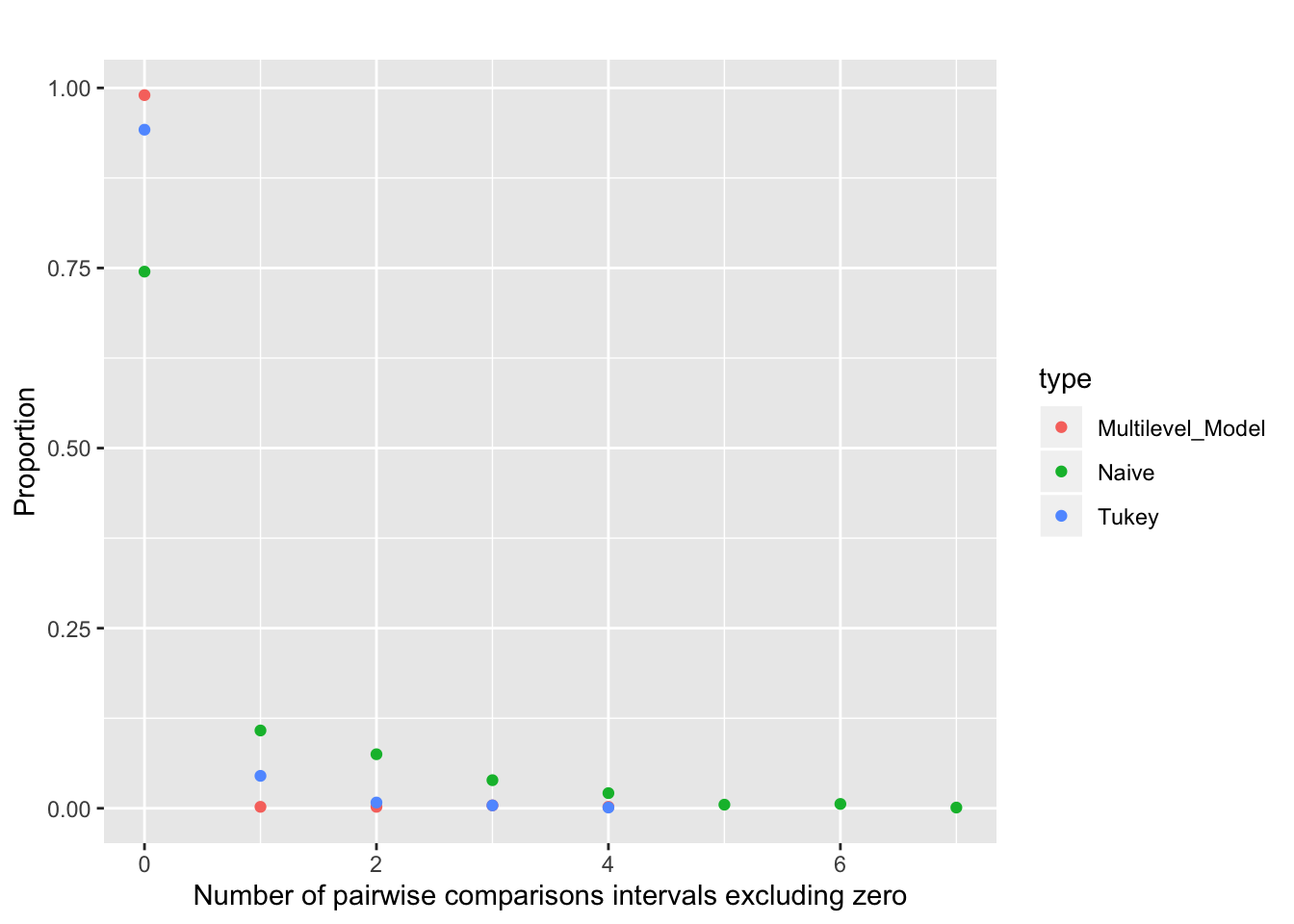
Conclusion
The above simulation excercise demonstrates that estimating effects under a multi-level framework is associated with a much lower false positive error rate, even when compared to the correction used in a frequentist inference. Since multilevel models are skeptical of extreme data, are able to “learn” from other groups, we are more likely to obtain precise intervals as compared to the traditional ANOVAs.
I would love to hear your thoughts on this and any comments are welcomed!
Thank you for reading!