Hello 2020! I’m going to start off this new year with a post that I’ve been meaning to put up for a while. It has nothing to do with statistics, but very much to do with my other love, the language R and it’s data manipulation libraries tidyr and data.table.
Introduction
For most of my work, the tidyverse set of packages get me where I want to be with the added ease of syntax, readibility and all the good stuff. But every now and then I’ll encounter a situation where I have to fall back on those saved bookmarks with data.table tutorials.
One of these was where I was dealing with ~ 20,000 groups with each group occuring ~15 times on an average. One of the measurements for these needed to be imputed by group i.e, one measurment was available per group, but this needed to be “filled” for the whole group. Yes, if you didn’t already guess it, tidyr::fill() is the way to go in a single line. This is exactly what I thought and set up my code and ran it.
My laptop ran for a whole day and it still hadn’t stopped running.
Enter data.table
I turned to the overlords of speed, the data.table library to possible speed it up, and in doing so learned that not only can you use pipes with data.tables, but also literally any function can be used within it! Using the .SD argument, you can pretty much use data.table in the same way as you would a tibble.
I set up my code to run, expecting to come back a few hours laters to see if it was finished running, but to my disbelief, it was done within a matter of minutes! The SAME function applied to a tibble ran for a day, but when using a data.table, done within minutes?!
Results
I had to confirm this finding wasn’t a fluke so I set out to run some simulations, and the results are, quite eye-opening. When the groups are in the 10s or the 100s, data.table performs marginally better, and that too a the millisecond level. No biggie - who even cares for a few milliseconds? But when the groups reach 5000, the difference is YUUUUUUGE - > ~ 200 fold difference, at the level of seconds… 7 seconds for a data.table to do the same thing that took tibble 26 minutes.
tests <- readRDS(here::here("static", "files", "tests_5000_groups.rds"))
tests <- set_names(tests, nm = c("10 groups", "100 groups", "1000 groups", "2000 groups", "5000 groups"))

purrr::map(tests, ~autoplot(.x))
## $`10 groups`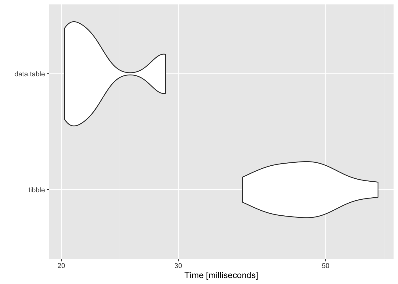
##
## $`100 groups`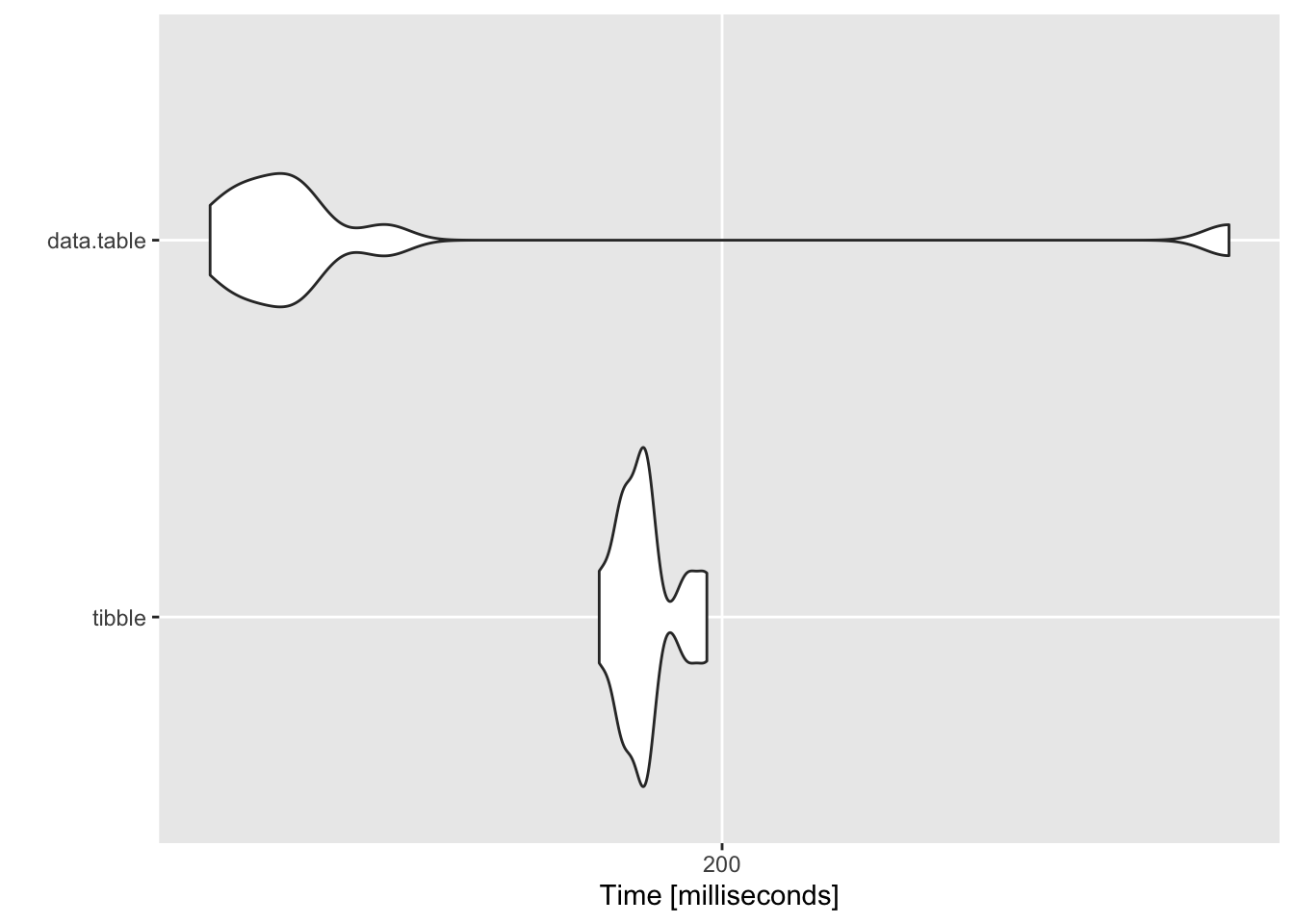
##
## $`1000 groups`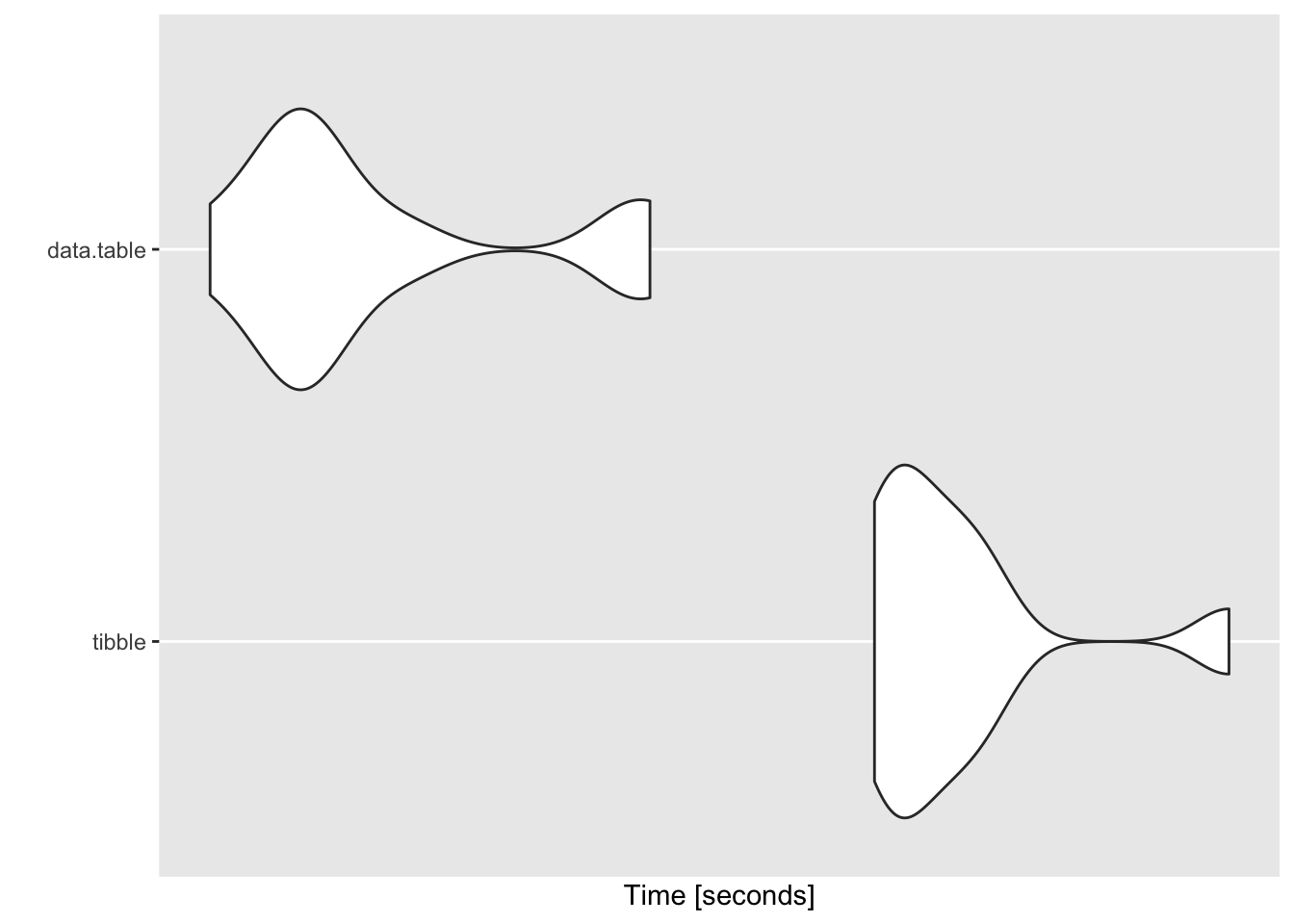
##
## $`2000 groups`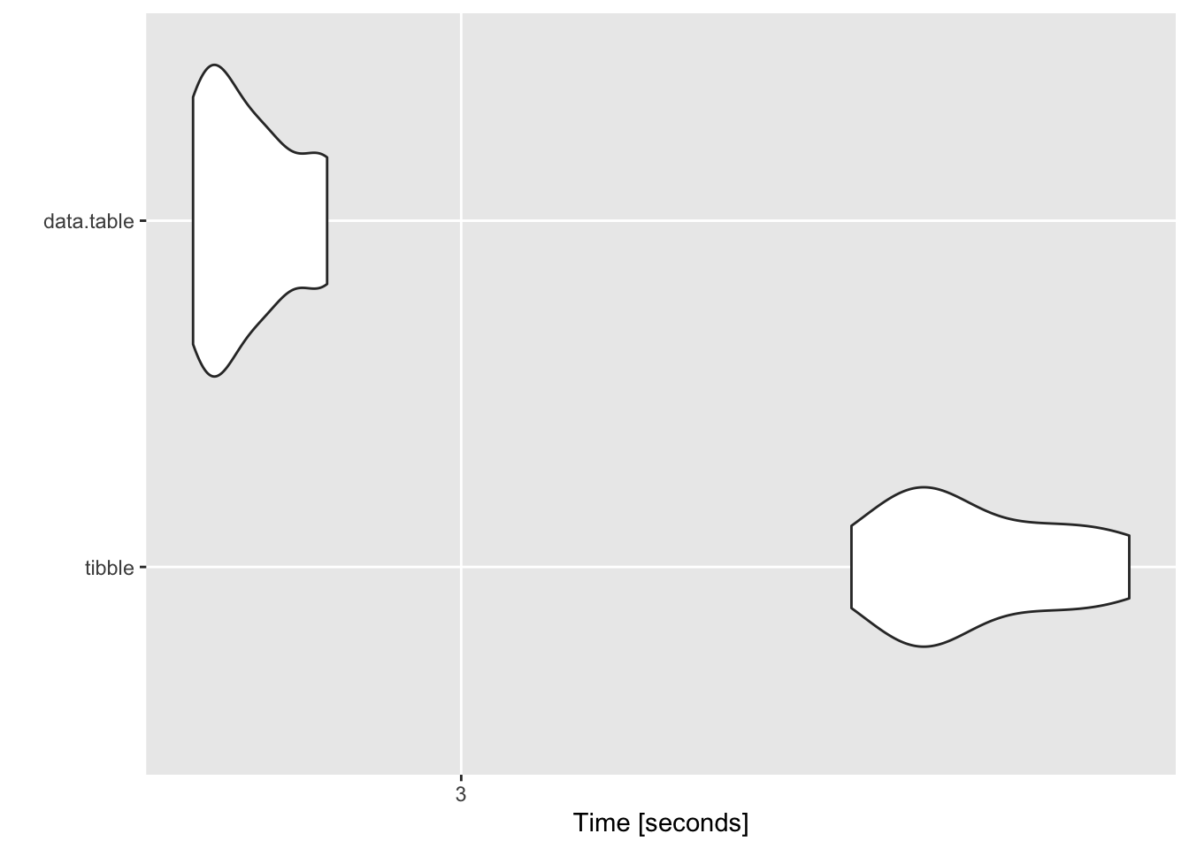
##
## $`5000 groups`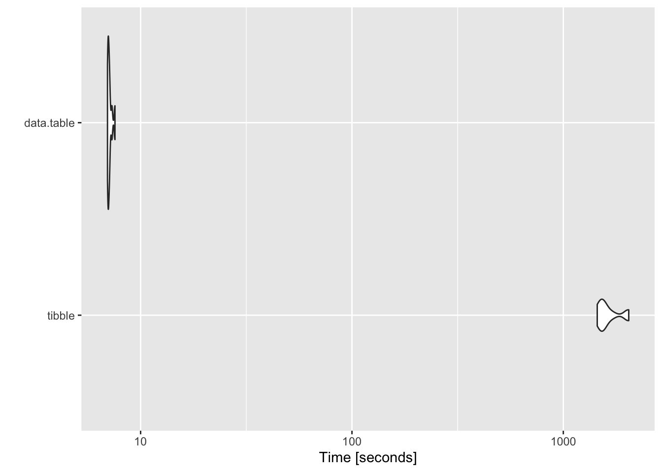
tests## $`10 groups`
## Unit: milliseconds
## expr min lq mean median uq max neval
## tibble 37.49481 41.98588 46.58438 46.50469 49.90171 59.94450 10
## data.table 20.22548 20.42626 22.69165 21.65140 22.78060 28.70793 10
## cld
## b
## a
##
## $`100 groups`
## Unit: milliseconds
## expr min lq mean median uq max neval
## tibble 184.7798 187.5413 190.2715 190.1950 190.4937 198.0482 10
## data.table 143.8182 147.0359 163.0706 150.7431 153.1045 277.2147 10
## cld
## b
## a
##
## $`1000 groups`
## Unit: seconds
## expr min lq mean median uq max neval
## tibble 1.687751 1.696000 1.726084 1.711365 1.735190 1.859891 10
## data.table 1.406881 1.435975 1.471199 1.449469 1.483755 1.587060 10
## cld
## b
## a
##
## $`2000 groups`
## Unit: seconds
## expr min lq mean median uq max neval
## tibble 3.317388 3.374256 3.426579 3.389765 3.487578 3.563575 10
## data.table 2.799702 2.814149 2.838442 2.826381 2.856391 2.898111 10
## cld
## b
## a
##
## $`5000 groups`
## Unit: seconds
## expr min lq mean median uq
## tibble 1447.198957 1500.951692 1640.659575 1559.728039 1705.000048
## data.table 6.970596 7.015401 7.129674 7.074186 7.150923
## max neval cld
## 2039.625297 10 b
## 7.563135 10 aThat’s a massive difference that can’t be ignored. When this number goes up to 10000 my laptop ran for hours at a stretch and I had to pull the plug on it because I had no idea how long it would take.
Code for simulation
Below is the simualtion I ran for the results above. I create a function that can create the specified number of groups and an associated measuremnt for each occurence of the group. The proportion of missing data in the measured variable can also be specified and randomly assigns missing values to the measurment.
The benchmarking for the fill function happens in the same function itself and it returns a data.frame with the benchmark results.
library(tidyverse)
library(microbenchmark)
library(data.table)


fill_benchmarking <- function(n = 1e5, groups = 1e2,
                              missing_proportion = 0.3, times = 1) {

  missing_var <- rnorm(n, 10, 5)
  ## this creates the proportion of missing data
  index <- rbinom(n, 1, missing_proportion)
  miising_var <- cbind(missing_var, index)
  ## create missing data
  missing_var <- ifelse(index == 1, NA, missing_var)

  ## create a grouping variable
  grouping_var <- as.character(rep(1:groups, each = n/groups))

  df <- tibble(missing_var = missing_var, grouping_var = grouping_var)

  ## this performs the benchmarking. The number of iterations can be specified by
  ## the argument times
  bm <- microbenchmark::microbenchmark(tibble =

                                  ## Use fill() on a tibble
                                  df <- df %>%
                                    group_by(grouping_var) %>%
                                    fill(., missing_var, .direction = "up") %>%
                                    fill(., missing_var, .direction = "down")

                                ,
                                ## Use fill() on a data.table
                                  data.table =
                                     dt <- df %>%
                                            setDT(.) %>%
                                           .[, fill(.SD, missing_var, .direction = "up"), by = "grouping_var"] %>%
                                           .[, fill(.SD, missing_var, .direction = "down"), by = "grouping_var"]
                              ,
                              times  = times)}
We iterate this function for 10 times over varying number of groups
tests <- purrr::map(c(10,100,1000, 2000, 5000), ~
                fill_benchmarking(groups = .x, times = 10))
saveRDS(tests, here::here("static", "files", "tests_5000_groups.rds"))
Conclusion
Going through this excercise taught me how to use tidyr verbs in a data.table, AND use pipes to keep the syntax clearer and distinct. But also, contrary to what I thought before, that a few milliseconds worth of speed increase isn’t important enough for me to spend time learning data.table, it really is a powerful library which provides unknowingly massive speed bumps as compared to a tibble, not just in the seconds but in minutes, which could be a gamechanger if you’re deploying real time applications.
sessioninfo::session_info()## ─ Session info ──────────────────────────────────────────────────────────
## setting value
## version R version 3.6.1 (2019-07-05)
## os macOS High Sierra 10.13.6
## system x86_64, darwin15.6.0
## ui X11
## language (EN)
## collate en_US.UTF-8
## ctype en_US.UTF-8
## tz America/Chicago
## date 2020-02-02
##
## ─ Packages ──────────────────────────────────────────────────────────────
## package * version date lib source
## assertthat 0.2.1 2019-03-21 [1] CRAN (R 3.6.0)
## backports 1.1.4 2019-04-10 [1] CRAN (R 3.6.0)
## blogdown 0.14 2019-07-13 [1] CRAN (R 3.6.0)
## bookdown 0.12 2019-07-11 [1] CRAN (R 3.6.0)
## broom 0.5.2 2019-04-07 [1] CRAN (R 3.6.0)
## cellranger 1.1.0 2016-07-27 [1] CRAN (R 3.6.0)
## cli 1.1.0 2019-03-19 [1] CRAN (R 3.6.0)
## codetools 0.2-16 2018-12-24 [1] CRAN (R 3.6.1)
## colorspace 1.4-1 2019-03-18 [1] CRAN (R 3.6.0)
## crayon 1.3.4 2017-09-16 [1] CRAN (R 3.6.0)
## data.table * 1.12.2 2019-04-07 [1] CRAN (R 3.6.0)
## digest 0.6.20 2019-07-04 [1] CRAN (R 3.6.0)
## dplyr * 0.8.3 2019-07-04 [1] CRAN (R 3.6.0)
## evaluate 0.14 2019-05-28 [1] CRAN (R 3.6.0)
## forcats * 0.4.0 2019-02-17 [1] CRAN (R 3.6.0)
## generics 0.0.2 2018-11-29 [1] CRAN (R 3.6.0)
## ggplot2 * 3.2.0 2019-06-16 [1] CRAN (R 3.6.0)
## glue 1.3.1 2019-03-12 [1] CRAN (R 3.6.0)
## gtable 0.3.0 2019-03-25 [1] CRAN (R 3.6.0)
## haven 2.1.1 2019-07-04 [1] CRAN (R 3.6.0)
## here 0.1 2017-05-28 [1] CRAN (R 3.6.0)
## hms 0.5.0 2019-07-09 [1] CRAN (R 3.6.0)
## htmltools 0.3.6 2017-04-28 [1] CRAN (R 3.6.0)
## httr 1.4.0 2018-12-11 [1] CRAN (R 3.6.0)
## jsonlite 1.6 2018-12-07 [1] CRAN (R 3.6.0)
## knitr 1.23 2019-05-18 [1] CRAN (R 3.6.0)
## lattice 0.20-38 2018-11-04 [1] CRAN (R 3.6.1)
## lazyeval 0.2.2 2019-03-15 [1] CRAN (R 3.6.0)
## lifecycle 0.1.0 2019-08-01 [1] CRAN (R 3.6.0)
## lubridate 1.7.4 2018-04-11 [1] CRAN (R 3.6.0)
## magrittr 1.5 2014-11-22 [1] CRAN (R 3.6.0)
## MASS 7.3-51.4 2019-03-31 [1] CRAN (R 3.6.1)
## Matrix 1.2-17 2019-03-22 [1] CRAN (R 3.6.1)
## microbenchmark * 1.4-7 2019-09-24 [1] CRAN (R 3.6.0)
## modelr 0.1.4 2019-02-18 [1] CRAN (R 3.6.0)
## multcomp 1.4-10 2019-03-05 [1] CRAN (R 3.6.0)
## munsell 0.5.0 2018-06-12 [1] CRAN (R 3.6.0)
## mvtnorm 1.0-11 2019-06-19 [1] CRAN (R 3.6.0)
## nlme 3.1-140 2019-05-12 [1] CRAN (R 3.6.1)
## pillar 1.4.2 2019-06-29 [1] CRAN (R 3.6.0)
## pkgconfig 2.0.2 2018-08-16 [1] CRAN (R 3.6.0)
## purrr * 0.3.2 2019-03-15 [1] CRAN (R 3.6.0)
## R6 2.4.0 2019-02-14 [1] CRAN (R 3.6.0)
## Rcpp 1.0.1 2019-03-17 [1] CRAN (R 3.6.0)
## readr * 1.3.1 2018-12-21 [1] CRAN (R 3.6.0)
## readxl 1.3.1 2019-03-13 [1] CRAN (R 3.6.0)
## rlang 0.4.0 2019-06-25 [1] CRAN (R 3.6.0)
## rmarkdown 1.14 2019-07-12 [1] CRAN (R 3.6.0)
## rprojroot 1.3-2 2018-01-03 [1] CRAN (R 3.6.0)
## rstudioapi 0.10 2019-03-19 [1] CRAN (R 3.6.0)
## rvest 0.3.4 2019-05-15 [1] CRAN (R 3.6.0)
## sandwich 2.5-1 2019-04-06 [1] CRAN (R 3.6.0)
## scales 1.0.0 2018-08-09 [1] CRAN (R 3.6.0)
## sessioninfo 1.1.1 2018-11-05 [1] CRAN (R 3.6.0)
## stringi 1.4.3 2019-03-12 [1] CRAN (R 3.6.0)
## stringr * 1.4.0 2019-02-10 [1] CRAN (R 3.6.0)
## survival 2.44-1.1 2019-04-01 [1] CRAN (R 3.6.1)
## TH.data 1.0-10 2019-01-21 [1] CRAN (R 3.6.0)
## tibble * 2.1.3 2019-06-06 [1] CRAN (R 3.6.0)
## tidyr * 1.0.2 2020-01-24 [1] CRAN (R 3.6.0)
## tidyselect 0.2.5 2018-10-11 [1] CRAN (R 3.6.0)
## tidyverse * 1.2.1 2017-11-14 [1] CRAN (R 3.6.0)
## vctrs 0.2.0 2019-07-05 [1] CRAN (R 3.6.0)
## withr 2.1.2 2018-03-15 [1] CRAN (R 3.6.0)
## xfun 0.8 2019-06-25 [1] CRAN (R 3.6.0)
## xml2 1.2.0 2018-01-24 [1] CRAN (R 3.6.0)
## yaml 2.2.0 2018-07-25 [1] CRAN (R 3.6.0)
## zeallot 0.1.0 2018-01-28 [1] CRAN (R 3.6.0)
## zoo 1.8-6 2019-05-28 [1] CRAN (R 3.6.0)
##
## [1] /Library/Frameworks/R.framework/Versions/3.6/Resources/library