Introduction
The original motivation for this post was to recreate an analysis in BDA (chapter 8), but as I started working through it, I realized it is an opportunity to write about several interesting concepts within the same framework. The overarching theme of this post covers
1. How to set up a multivariate logistic regression (not a multinomial or multivariable)
1. How to set priors for Generalized Linear Models
3. Hierarchical Models and Shrinkage of parameters
What will you learn from this post?
My goal is that by the end of this post, you’ll be able to
1. Run prior predictive simulations for logistic regression models and hopefully I can convince you why using default priors or uninformative priors is generally a bad idea.
2. Visualize shrinkage in the context of hierarchical models.
Problem Set-up
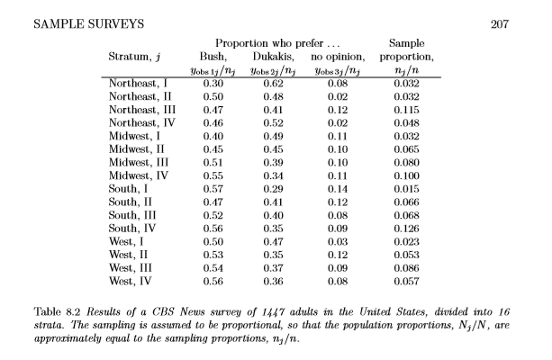
The data set for this problem comes from the chapter on Modeling for accounting in data collection process, where Gelman et al talk about accounting the data collection process into the model set-up. A stratified random sampling opinion poll was conducted and data collected from 16 strata across the country.
There are two parameters of interest for this analysis -
- Proportion of people voting bush (of the people who had an opinion) - \[ \alpha \ _1j \]
- Proportion of people that gave an opinion - \[ \alpha \ _2j \]
Both of these can be derived from the above data. In addition, we know the total number of people samples (n = 1447), so we use the sample_proportion to calculate how many people were sampled in each strata. (we’ll later use this to convert the data into a long form format)
Sample Survey
library(tidyverse)
library(brms)
library(tidybayes)
Data
df_raw <- tibble::tibble(stratum = c("northeast, I", "northeast,II","northeast,III","northeast,IV",
             "midwest,I","midwest,II","midwest,III","midwest,IV",
             "south,I","south,II","south,III","south,IV",
             "west,I","west,II","west,III","west,IV"),
                     proportion_bush =  c(0.30,0.5,0.47,0.46,0.40,0.45,0.51,0.55,0.57,0.47,0.52,0.56,0.50,
                      0.53,0.54,0.53),
                     proportion_dukakis = c(0.62,0.48,0.41,0.52,0.49,0.45,0.39,0.34,0.29,0.41,0.40,
                        0.35,0.47,0.35,0.37,0.36),
                     proportion_no_opinion = c(0.08,0.02,0.12,0.02,0.11,0.10,0.10,0.11,0.14,0.12,
                            0.08,0.09,0.03,0.12,0.09,0.08),
                     sample_proportion = c(0.032,0.032,0.115,0.048,0.032,0.065,0.080,0.100,0.015,0.066,0.068,
                       0.126,0.023,0.053,0.086,0.057))
Create the two parameters of interest
df <- df_raw %>%
  dplyr::mutate(a_1 = proportion_bush/(proportion_bush + proportion_dukakis)) %>%
  dplyr::mutate(a_2 = 1 - proportion_no_opinion) %>%
  dplyr::mutate(sampled_nj = round(sample_proportion*1447))

df <- df %>%
  mutate(a_1_count = round(a_1*sampled_nj),
         a_2_count = round(a_2*sampled_nj))
df %>%
knitr::kable()| stratum | proportion_bush | proportion_dukakis | proportion_no_opinion | sample_proportion | a_1 | a_2 | sampled_nj | a_1_count | a_2_count |
|---|---|---|---|---|---|---|---|---|---|
| northeast, I | 0.30 | 0.62 | 0.08 | 0.032 | 0.3260870 | 0.92 | 46 | 15 | 42 |
| northeast,II | 0.50 | 0.48 | 0.02 | 0.032 | 0.5102041 | 0.98 | 46 | 23 | 45 |
| northeast,III | 0.47 | 0.41 | 0.12 | 0.115 | 0.5340909 | 0.88 | 166 | 89 | 146 |
| northeast,IV | 0.46 | 0.52 | 0.02 | 0.048 | 0.4693878 | 0.98 | 69 | 32 | 68 |
| midwest,I | 0.40 | 0.49 | 0.11 | 0.032 | 0.4494382 | 0.89 | 46 | 21 | 41 |
| midwest,II | 0.45 | 0.45 | 0.10 | 0.065 | 0.5000000 | 0.90 | 94 | 47 | 85 |
| midwest,III | 0.51 | 0.39 | 0.10 | 0.080 | 0.5666667 | 0.90 | 116 | 66 | 104 |
| midwest,IV | 0.55 | 0.34 | 0.11 | 0.100 | 0.6179775 | 0.89 | 145 | 90 | 129 |
| south,I | 0.57 | 0.29 | 0.14 | 0.015 | 0.6627907 | 0.86 | 22 | 15 | 19 |
| south,II | 0.47 | 0.41 | 0.12 | 0.066 | 0.5340909 | 0.88 | 96 | 51 | 84 |
| south,III | 0.52 | 0.40 | 0.08 | 0.068 | 0.5652174 | 0.92 | 98 | 55 | 90 |
| south,IV | 0.56 | 0.35 | 0.09 | 0.126 | 0.6153846 | 0.91 | 182 | 112 | 166 |
| west,I | 0.50 | 0.47 | 0.03 | 0.023 | 0.5154639 | 0.97 | 33 | 17 | 32 |
| west,II | 0.53 | 0.35 | 0.12 | 0.053 | 0.6022727 | 0.88 | 77 | 46 | 68 |
| west,III | 0.54 | 0.37 | 0.09 | 0.086 | 0.5934066 | 0.91 | 124 | 74 | 113 |
| west,IV | 0.53 | 0.36 | 0.08 | 0.057 | 0.5955056 | 0.92 | 82 | 49 | 75 |
Transform to long form
Let’s transform this into a long form data set, where responses are classified as 0 or 1.
## The following code chunk makes use of purrr and list columns to generate 0s and 1s
## The map2 takes in as vectors two things - the sampled people in each strata and
## the proportion of people for each parameter of interest

df_sub <- df %>%
  select(stratum, sampled_nj, a_1_count, a_2_count) %>%
  mutate(strata = map2(as_vector(.['stratum']), 1:16,
                       ~ c(rep(.x, times = df[.y, 'sampled_nj'])))) %>%
  mutate(a_1_binary = map2(as_vector(.['sampled_nj']),
                              as_vector(.['a_1_count']),
                              ~ c(rep(0, times = .x - .y), rep(1, times = .y)))) %>%
  mutate(a_2_binary = map2(as_vector(.['sampled_nj']),
                              as_vector(.['a_2_count']),
                              ~ c(rep(0, times = .x - .y), rep(1, times = .y))))

## This just unnests the list columns

df_long <- df_sub %>%
  select(strata, a_1_binary, a_2_binary) %>%
  unnest(cols = c(strata, a_1_binary, a_2_binary))

## See what the data looks like

df_long %>%
  sample_n(10) %>%
knitr::kable()| strata | a_1_binary | a_2_binary |
|---|---|---|
| northeast,IV | 1 | 1 |
| west,IV | 0 | 1 |
| northeast,III | 0 | 0 |
| west,III | 1 | 1 |
| midwest,IV | 0 | 0 |
| northeast, I | 0 | 1 |
| midwest,III | 0 | 1 |
| midwest,II | 1 | 1 |
| midwest,I | 0 | 0 |
| west,III | 1 | 1 |
Hierarchical Model
Now that we have our data set up the way we’d like, we move on to modeling it. The natural choice for this is to model it as a hierarchical model - each strata is assumed to be exchangeable. For more on Hierarchical models and the set up, Chapter 5 in BDA is an excellent resources to know the guts of how these models work. Instead of modeling each strata as a fixed effect, we model these strata to come from the same population distribution. The estimate for each strata learns information from the other strata too.
Prior Predictive Simulation
Generalized Linear Models are interaction models even if you haven’t specified any interactions. Priors that may make sense on the logit scale don’t always make sense on the probability scale. brms by default uses student_t(3, 0, 10) priors for the population level effects in hierarchical models. These are called “weakly informative priors” and more often than not help with efficient sampling of the posterior space.
Even with small amount data, the likelihood would take over and these “weakly informative priors” won’t affect our inferences, but as you start fitting more complex models, putting sensible informative priors on your parameters is more likely to lead to better sampling.
Here we’ll look at what happens if we simulate data from the default priors and have a look at the plausible outcome space before observing the data
m1.prior <- fit1 <- brm(mvbind(a_1_binary, a_2_binary) ~ (1|p|strata), data = df_long,
                  family = bernoulli, sample_prior = "only",
                  chains = 4, cores = 2 )
saveRDS(m1.prior, here::here("static", "files", "m1_prior.rds"))
Before observing the data, what is our prior belief about people voting for bush on average across the whole country?
WOWZA! The default student_t(3, 0, 10) priors puts almost all mass in either extremes, which says, we either expect a large majority to vote for bush or a large majority not to vote for bush. That seems like a pretty unreasonable prior belief to keep.
One of the criticisms that people have of bayesian statistics is that it is “subjective” and an often touted counter point is, to just use non-informative priors. Below is a classic example of why using non-informative priors does more harm than good.
posterior_samples(m1.prior) %>%
  select(1) %>%
  mutate(prior_bush = inv_logit_scaled(b_a1binary_Intercept)) %>%
  ggplot(.,aes(prior_bush)) + geom_density() +
  labs(title = "Prior Probability of Voting for Bush",
       x = "Probability",y = "Density")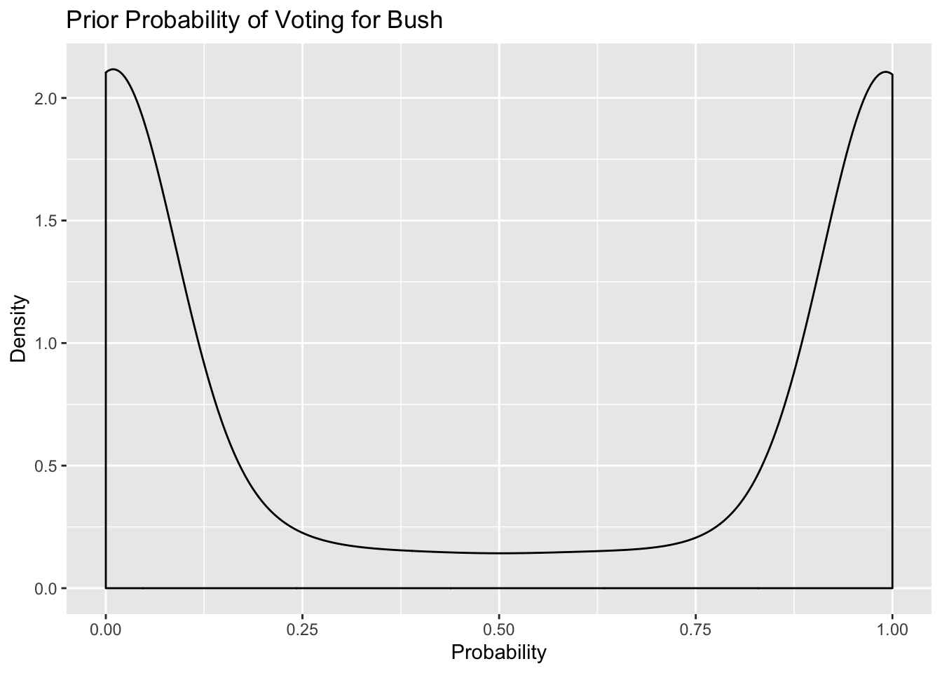
We could do a similar prior simulation for each region, and unsurprisingly, they have a similar distribution -
tidybayes::add_linpred_draws(newdata = df_long[1, 'strata'], m1.prior) %>%
  filter(.category == "a1binary") %>%
ggplot(.,aes(.value)) + geom_density() 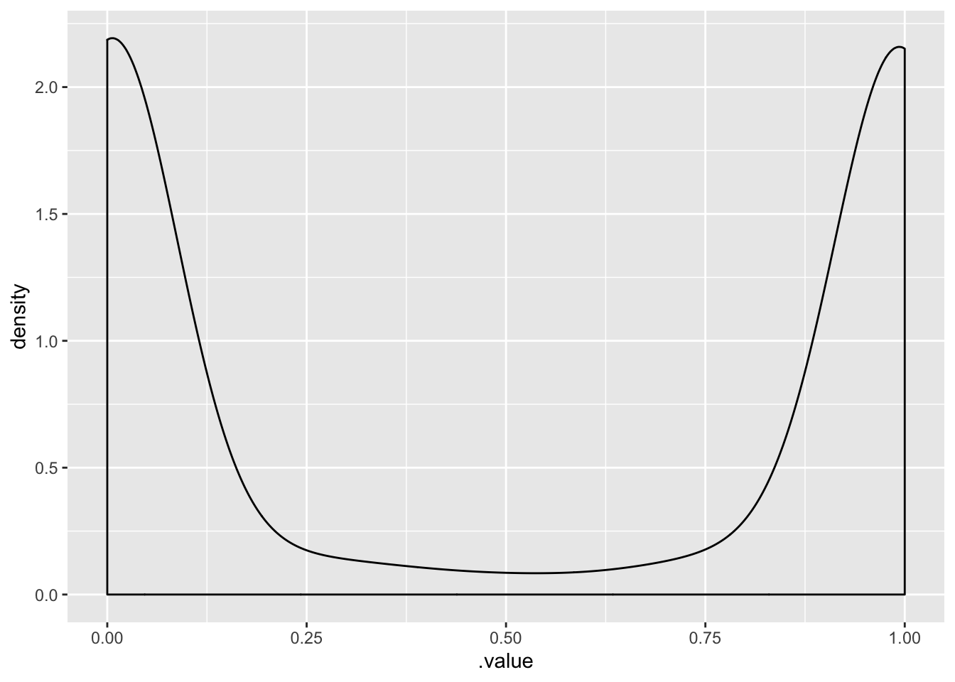
Correlation - Before observing the data, what is our prior belief about the correlation between voting bush and having an opinion?
It’s quite uniformly distributed.
posterior_samples(m1.prior) %>%
  select(cor_strata__a1binary_Intercept__a2binary_Intercept) %>%
  ggplot(.,aes(cor_strata__a1binary_Intercept__a2binary_Intercept)) +
geom_density() 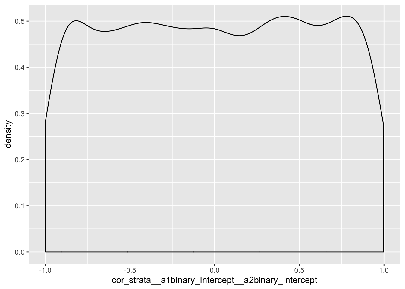
Regularizing Priors
Regularize the priors some and simulate the prior predictive distribution
m2.prior <- brm(mvbind(a_1_binary, a_2_binary) ~ (1|p|strata), data = df_long,
                  family = bernoulli, sample_prior = "only",
                  chains = 4, cores = 2,
                  prior = c(prior(student_t(3, 0, 1), class = sd, resp = a1binary),
                            prior(student_t(3, 0, 1), class = sd, resp = a2binary),
                  prior(student_t(3, 0, 1), class = Intercept),
                  prior(lkj(2), class = cor)))
saveRDS(m2.prior, here::here("static", "files", "m2_prior.rds"))
Prior probability
These prior distributions look much more reasonable - the average probability is centered at 0.5 and puts equal mass both sides. In addition, the probability of voting in the Northeast, I region is uniformly distributed - we may want to tighten those priors a bit more. Let’s do that in the next step.
Also, the distribution of correlation is much more reasonable - we don’t’ expect very strong correlations i.e it isn’t our belief that a high proportion of people having an opinion will also end up voting for bush or vice versa.
posterior_samples(m2.prior) %>%
  select(1) %>%
  mutate(prior_bush = inv_logit_scaled(b_a1binary_Intercept)) %>%
  ggplot(.,aes(prior_bush)) + geom_density() + labs(title = "Prior Probability of Voting for Bush",
                                                    x = "Probability",
                                                    y = "Density")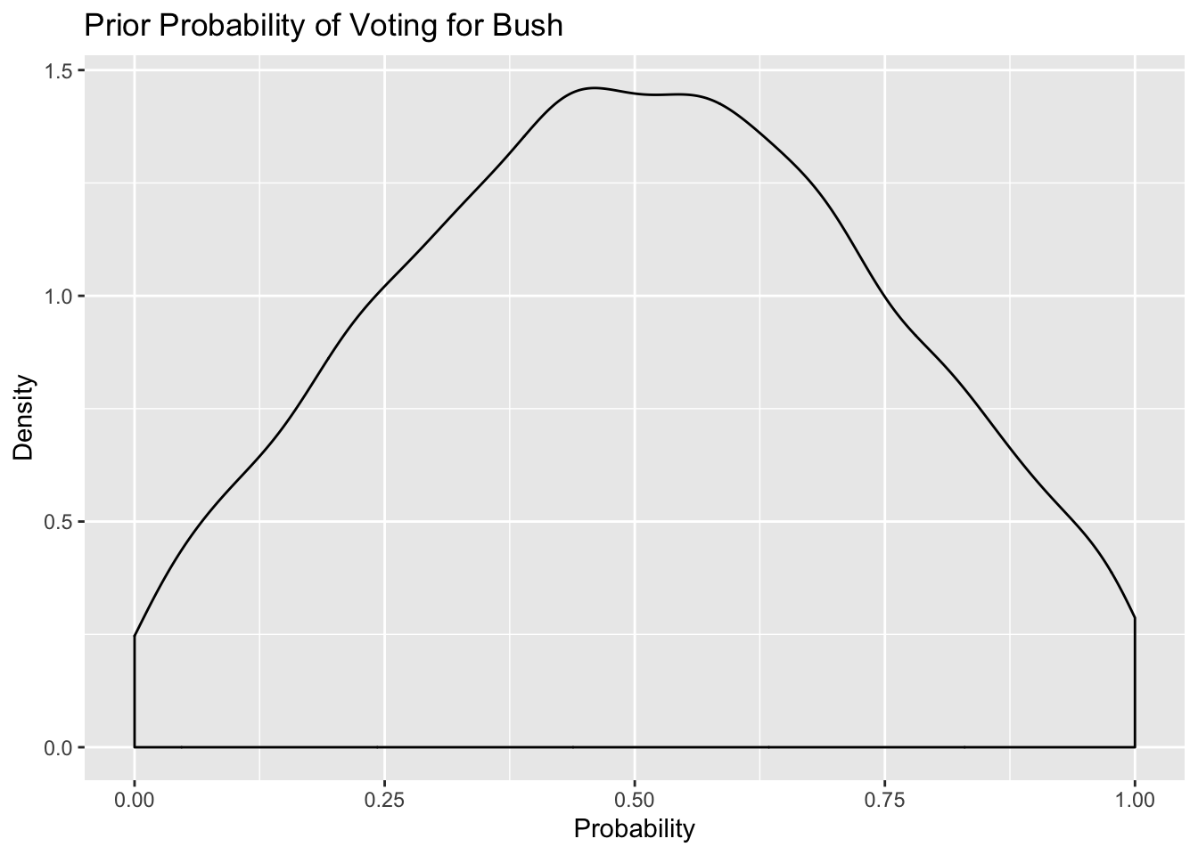
tidybayes::add_linpred_draws(newdata = df_long[1, 'strata'], m2.prior) %>%
  filter(.category == "a1binary") %>%
ggplot(.,aes(.value)) + geom_density() + labs(title = "Probability of Voting Bush in Northeast, I") 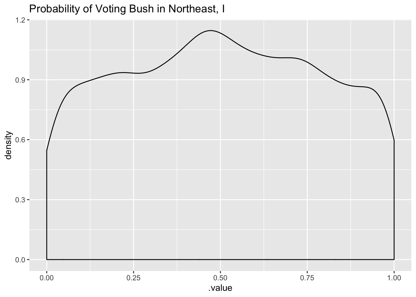
posterior_samples(m2.prior) %>%
  select(cor_strata__a1binary_Intercept__a2binary_Intercept) %>%
  ggplot(.,aes(cor_strata__a1binary_Intercept__a2binary_Intercept)) +
geom_density() + labs(title = "Prior Distribution of Correlation") 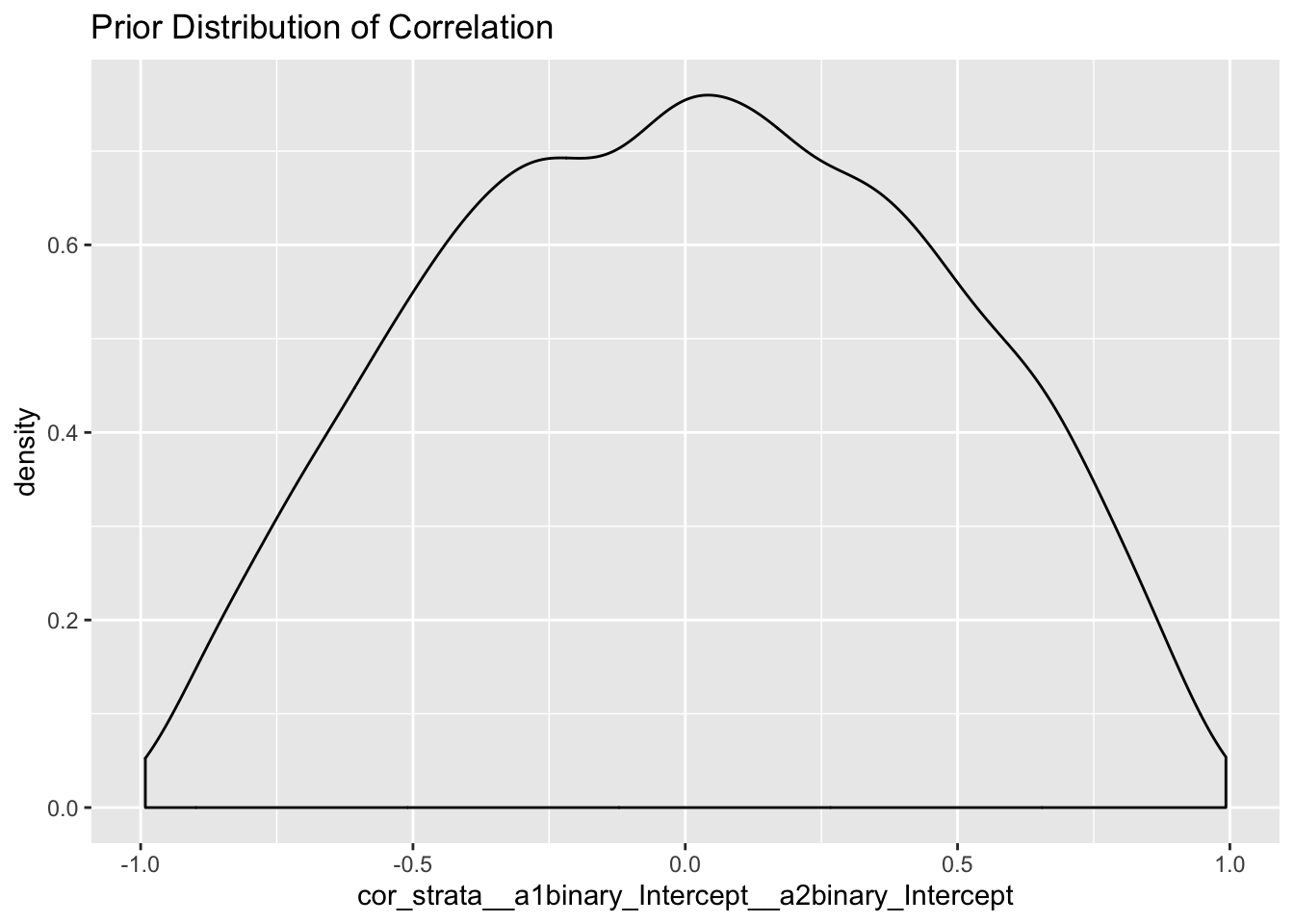
Even More Regularizing Priors for Regions
m3.prior <- fit1 <- brm(mvbind(a_1_binary, a_2_binary) ~ (1|p|strata), data = df_long,
                  family = bernoulli, sample_prior = "only",
                  chains = 4, cores = 2,
                  prior = c(prior(student_t(3, 0, 0.5), class = sd, resp = a1binary),
                            prior(student_t(3, 0, 0.5), class = sd, resp = a2binary),
                  prior(student_t(3, 0, 1), class = Intercept),
                  prior(lkj(2), class = cor)))
saveRDS(m3.prior, here::here("static", "files", "m3_prior.rds"))
Prior probability
posterior_samples(m3.prior) %>%
  select(1) %>%
  mutate(prior_bush = inv_logit_scaled(b_a1binary_Intercept)) %>%
  ggplot(.,aes(prior_bush)) + geom_density() +
  labs(title = "Prior Probability of Voting for Bush",
       x = "Probability", y = "Density")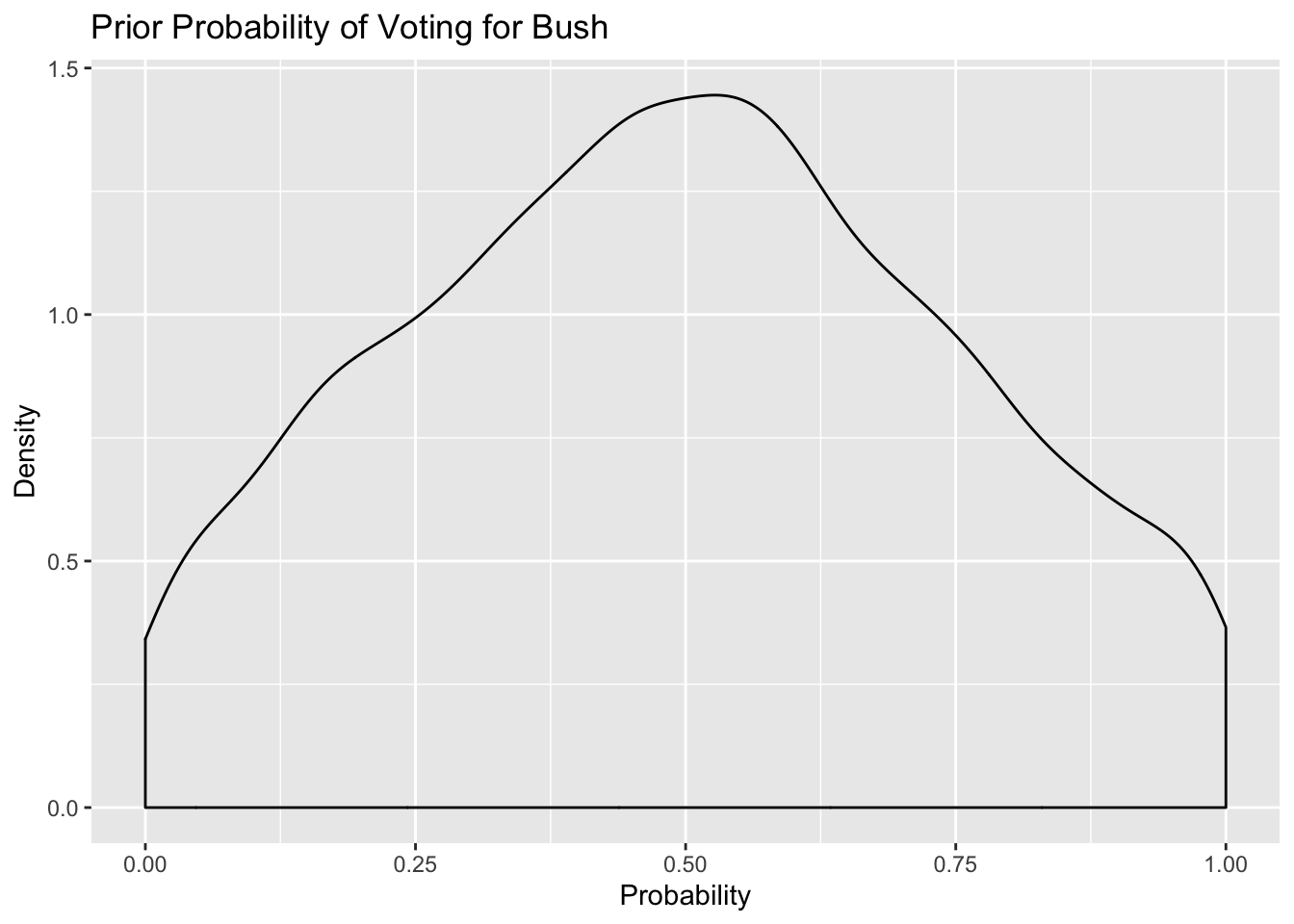
tidybayes::add_linpred_draws(newdata = df_long[1, 'strata'], m3.prior) %>%
  filter(.category == "a1binary") %>%
  ggplot(.,aes(.value)) + geom_density() +
  labs(title = "Probability of Voting Bush in Northeast, I")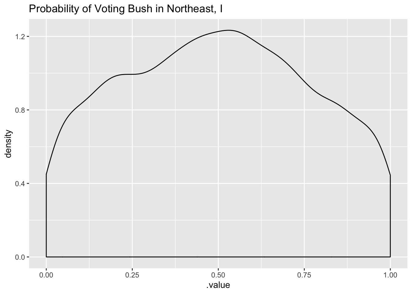
Separate Priors
Now say for instance, we don’t have prior beliefs on proportion of people voting for bush, but we do have an idea of whether or not people will give an opinion or not. Recall, the a_2_binary is the proportion of people who gave an opinion. It is unlikely that a large proportion of people will NOT give an opinion - political science majors would be much better suited to answer this question, but I’ll go out on a limp and say that it is much more likely that more than 50 % of the population will give an opinion - so I’d want a prior that puts much more weight towards the right as opposed to the left.
m4.prior <- brm(mvbind(a_1_binary, a_2_binary) ~ (1|p|strata), data = df_long,
                  family = bernoulli, sample_prior = "only",
                  chains = 4, cores = 2,
                  prior = c(prior(student_t(3, 0, 0.5), class = sd, resp = a1binary),
                            prior(student_t(3, 0, 0.5), class = sd, resp = a2binary),
                  prior(student_t(3, 0, 1), class = Intercept, resp = a1binary),
                  prior(student_t(3, 2, 1), class = Intercept, resp = a2binary),
                  prior(lkj(2), class = cor)))
saveRDS(m4.prior, here::here("static", "files", "m4_prior.rds"))
Visualize the second parameter - proportion of people giving an opinion
posterior_samples(m4.prior) %>%
  select(b_a2binary_Intercept) %>%
  mutate(prior_bush = inv_logit_scaled(b_a2binary_Intercept)) %>%
  ggplot(.,aes(prior_bush)) + geom_density() +
  labs(title = "Prior Probability of Giving an Opinion on Average",
       x = "Probability",y = "Density")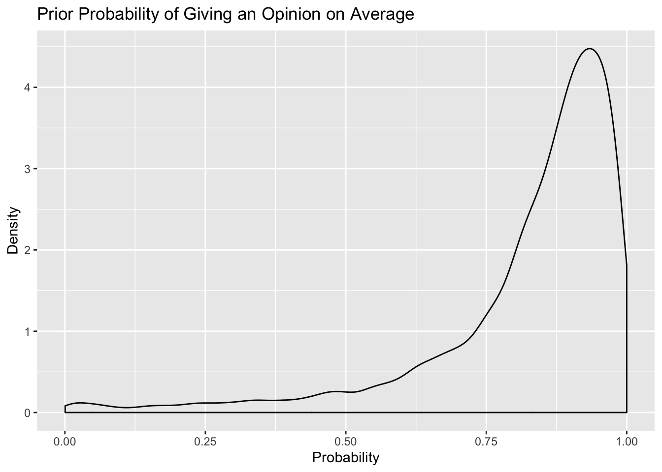
tidybayes::add_linpred_draws(newdata = df_long[6, 'strata'], m4.prior) %>%
  filter(.category == "a1binary") %>%
  ggplot(.,aes(.value)) + geom_density() +
labs(title = "Probability of Giving an Opinion in Northeast, I") 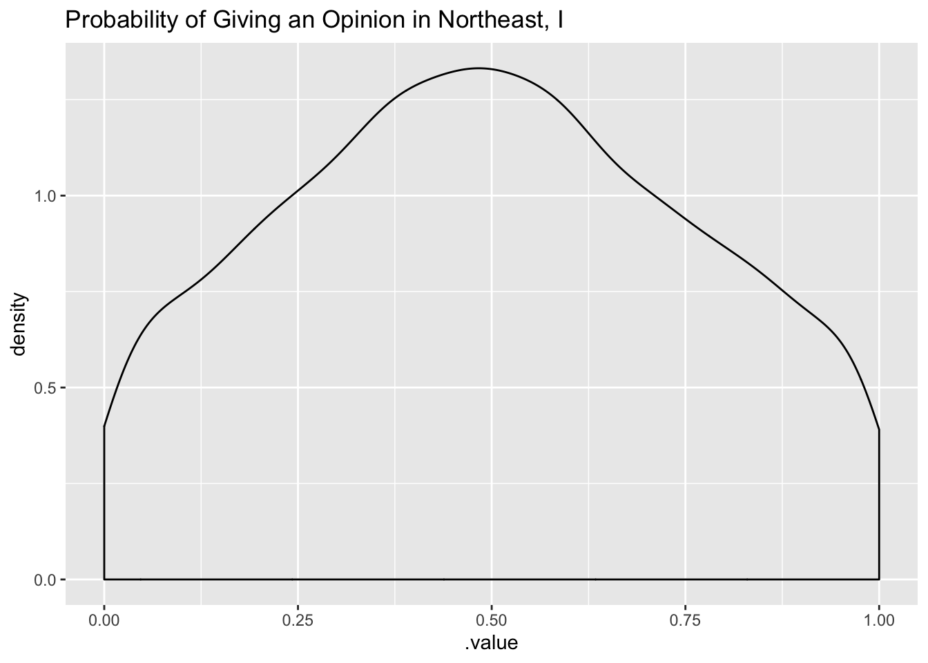
Posterior Distribution
Let’s go ahead with the priors set in model m4.prior - one of the key elements of bayesian analysis is sensitivity analysis. We can change our priors and see how inferences in the posterior distribution change.
## posterior
m1.posterior <- brm(mvbind(a_1_binary, a_2_binary) ~ (1|p|strata), data = df_long,
                  family = bernoulli,
                  chains = 4, cores = 4,
                  prior = c(prior(student_t(3, 0, 0.5), class = sd, resp = a1binary),
                            prior(student_t(3, 0, 0.5), class = sd, resp = a2binary),
                  prior(student_t(3, 0, 1), class = Intercept, resp = a1binary),
                  prior(student_t(3, 2, 1), class = Intercept, resp = a2binary),
                  prior(lkj(2), class = cor)))
saveRDS(m1.posterior, here::here("static", "files", "m1_posterior.rds"))
Posterior Checks
pp_check(m1.posterior, nsamples = 100, resp = "a1binary")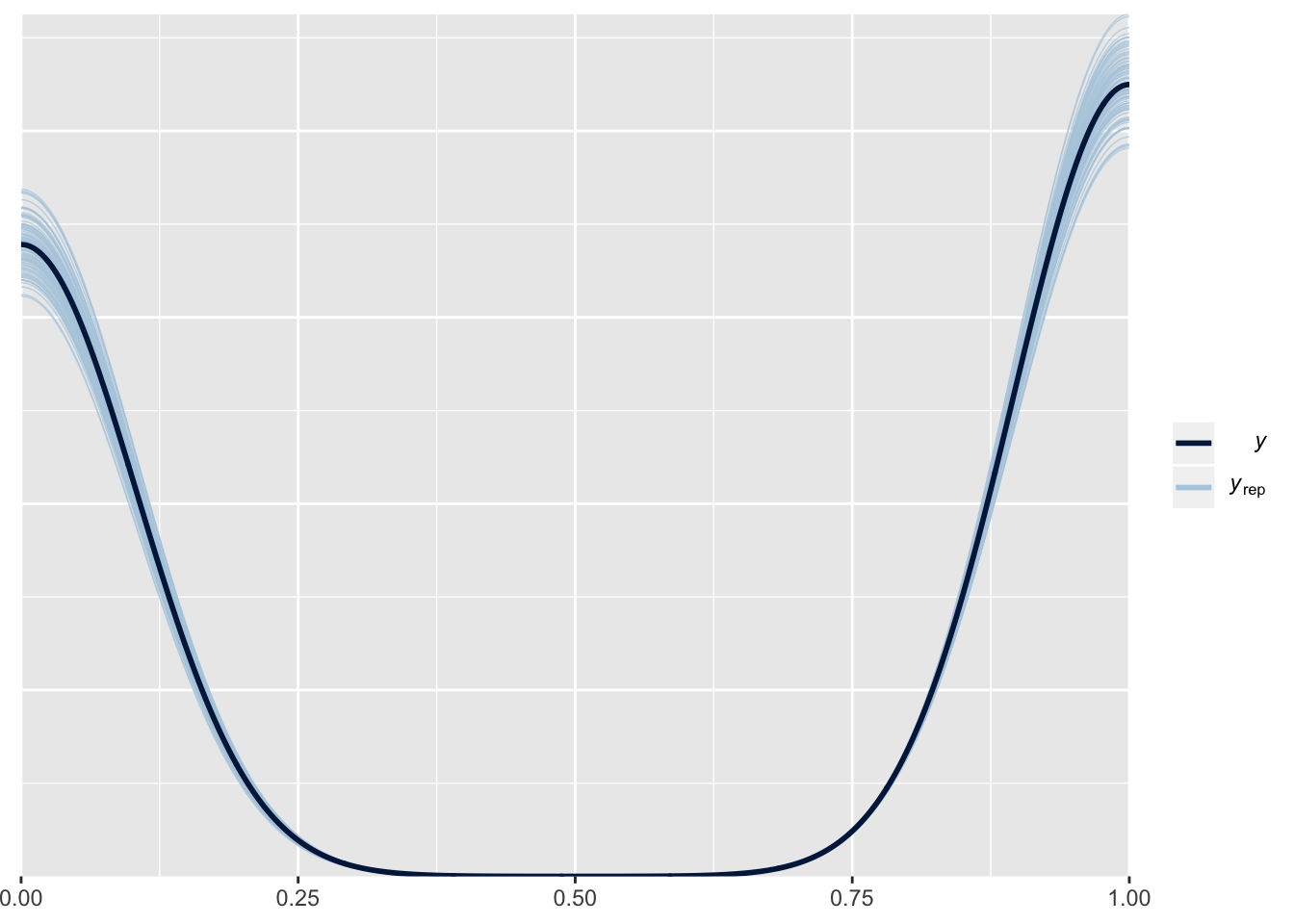
pp_check(m1.posterior, nsamples = 100, resp = "a2binary") 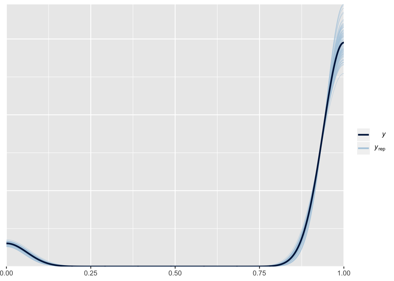
new_d <- df_long %>%
  select(strata) %>%
  distinct()
tidybayes::add_linpred_draws(newdata = new_d, m1.posterior, seed = 123) %>%
median_qi() %>%
ggplot(., aes(.value, strata)) + geom_pointintervalh() +
facet_wrap(vars(group = .category)) 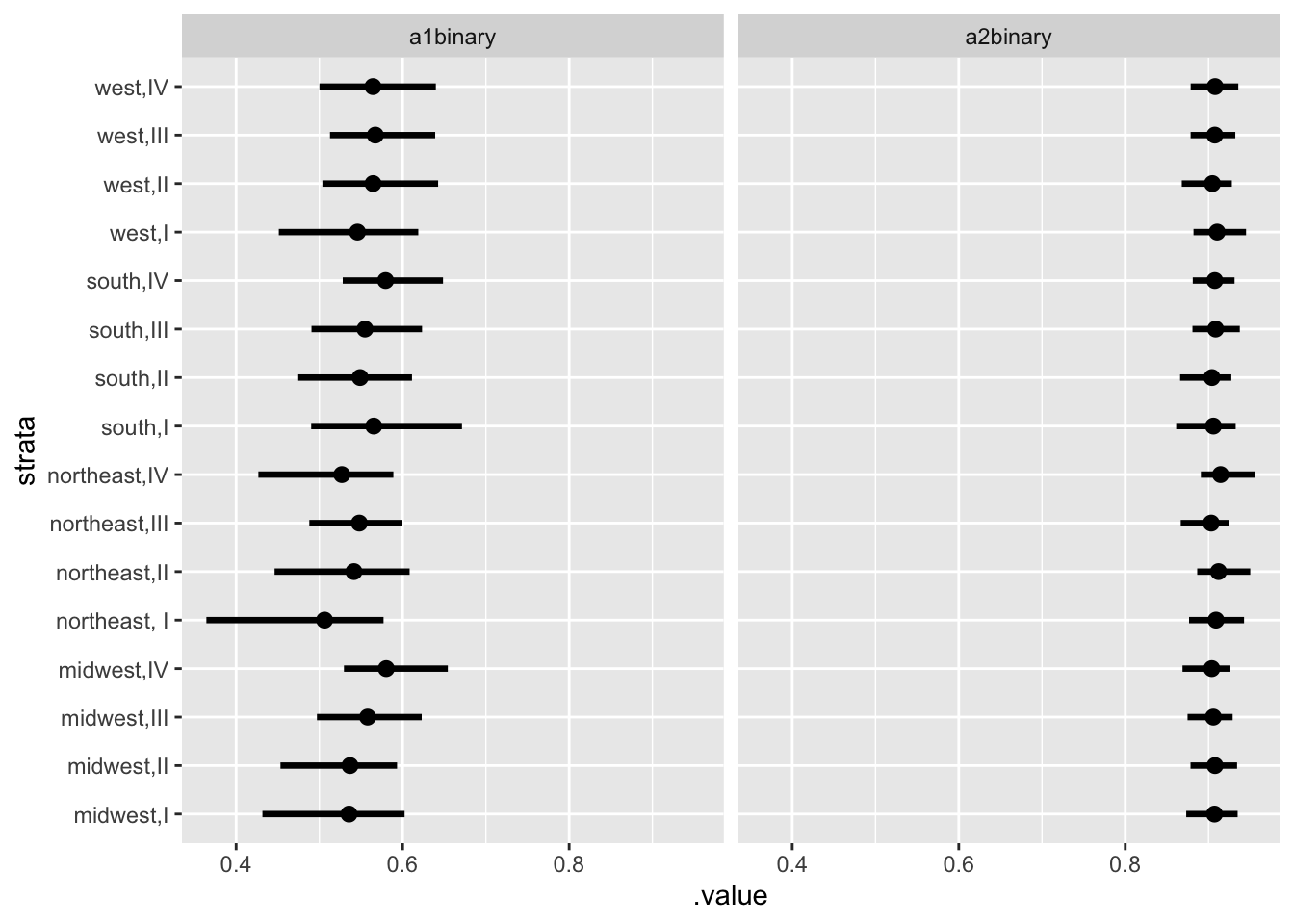
Shrinkage
Model checking doesn’t stop at the posterior predictive checks, one should ALWAYS be skeptical of the model results even if you’re satisfied at that stage. Another valuable tool is to simply compare the raw data estimates with the posterior predictions, and note where the results are different and where they are the same.
Hierarchical Models “shrink” estimates towards the grand mean, unless there’s strong evidence not to. That in fact is one of the major advantages, as it protects us from concluding groups are different, when in fact they’re not (multiple comparisons discussed in earlier post).
We see that quite clearly in the plot below - for both estimates, extreme values are shrunk towards the center of the population distribution.
An apple doesn’t fall too far away from the tree, so unless we have strong evidence that it is a peach, we treat it as being from the apple tree closest to it.
tidybayes::add_linpred_draws(newdata = new_d, m1.posterior, seed = 123) %>%
  mean_qi() %>%
  filter(.category == "a1binary") %>%
  inner_join(df_raw, by = c("strata" = "stratum")) %>%
  ggplot(., aes(.value, strata)) + geom_pointintervalh() +
  geom_point(aes(proportion_bush), color = "red") + labs(title = "Estimated Proportion Voting for Bush in Each Region")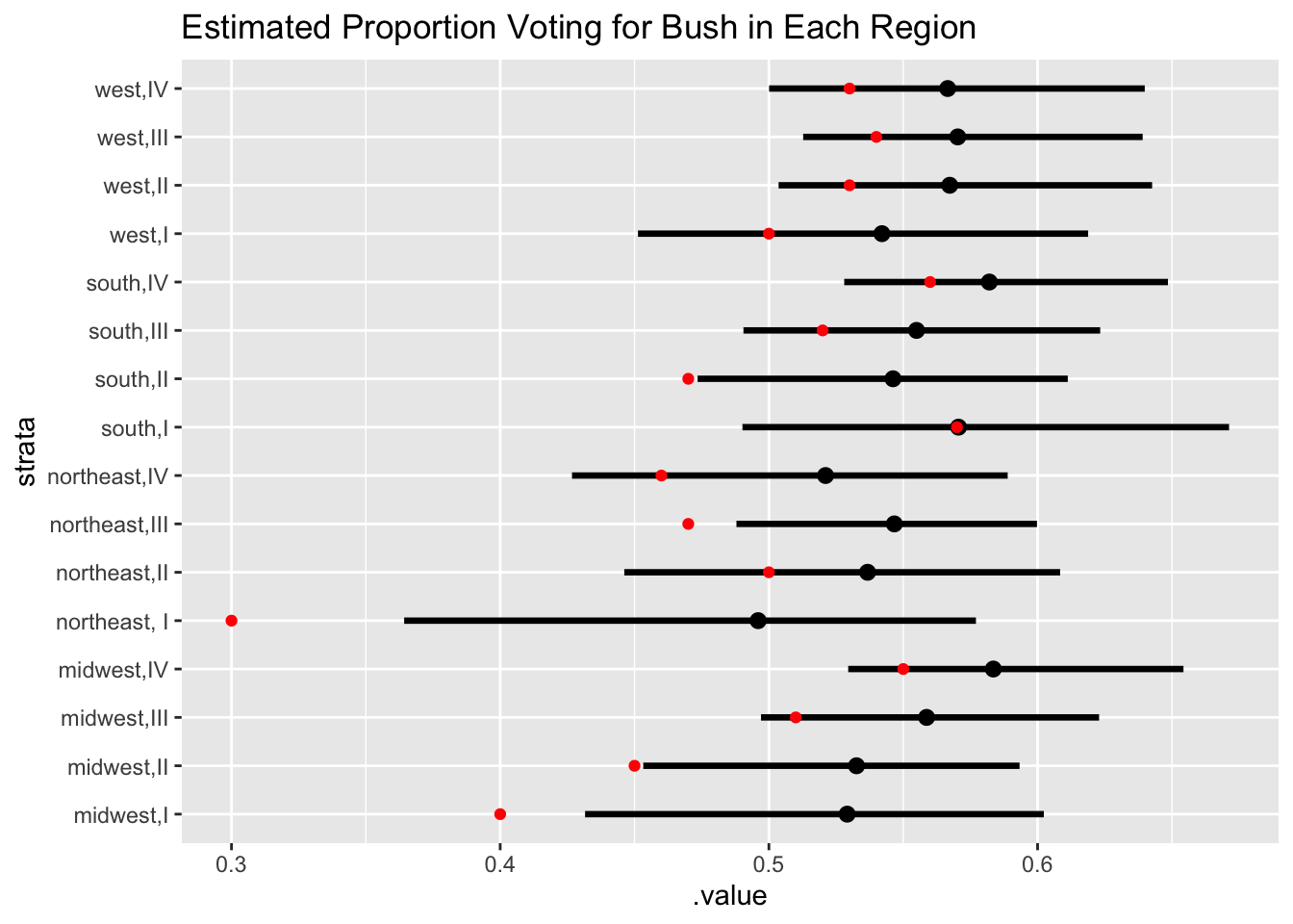
tidybayes::add_linpred_draws(newdata = new_d, m1.posterior, seed = 123) %>%
  mean_qi() %>%
  filter(.category == "a2binary") %>%
  inner_join(df_raw, by = c("strata" = "stratum")) %>%
  ggplot(., aes(.value, strata)) + geom_pointintervalh() +
  geom_point(aes(1 -  proportion_no_opinion), color = "red") + labs(title = "Estimated Proportion having an opinion")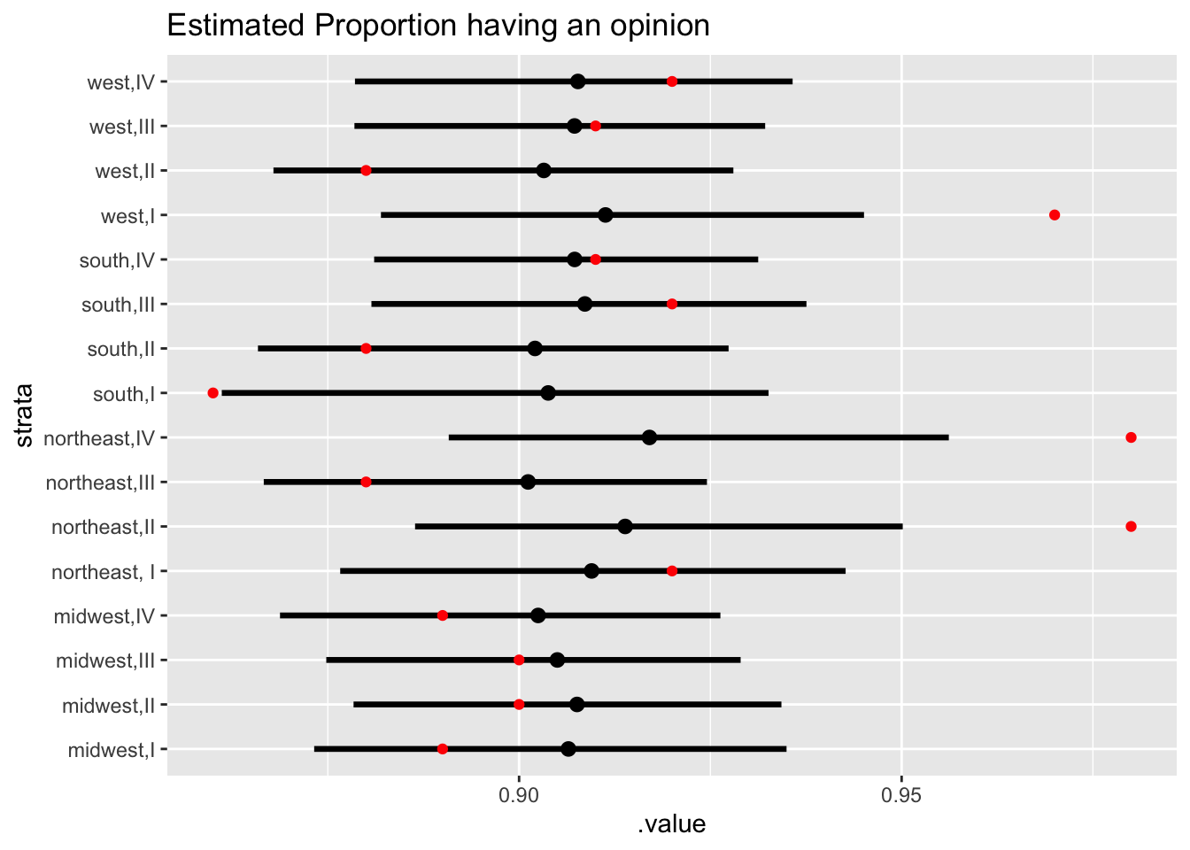
The northeast, I region has a lot more shrinkage than the others, which is a cause for concern. At this point, it is imperative to run some checks to ensure the validity of the model. And this will be our topic for the next post! How to check your model fit by looking at the implied posterior predictions.
Conclusion
This case study isn’t focused on one particular concept, but rather, how different aspects of bayesian inference are used to build models. We saw how even weakly informative priors can have severe consequences on the outcome of interest in the case of generalized linear models. It is imperative to simulate data from you priors and ensure that even if you’re not putting priors that encode your beliefs, they should still lead to an outcome space that is somewhat plausible. It is highly improbable for people to give either candidate a landslide victory, so we should set priors that don’t put all of the mass at the extremes.
Another takeaway from this was how to implement a multivariate logistic regression in brms - as noted above this is very straightforward to implement, thanks to Paul Berkner. In addition, we saw how modeling the data as a hierarchical structure leads to regularized estimates.
